Model predictive control is like playing chess, at ,each time step, you choose the best strategy to win. In this process, you make prediction based on current situation.
Model predictive control (MPC), also known as dynamical matrix control (DMC), generalized predictive control (GPC) or receding horizon control (RHC), is an online control algorithm based on numerically solving an optimal problem at each step. This article gives a summarization about model predictive control strategy. It is mainly a summarization about reference 2
Why MPC
- Intuitive concept, easy to understand and implement
- Systematic handling of constrains
- Can handle MIMO and dead-time without modification
- Feed forward to make good use of future target information
- Handling challenging dynamics (unlike PID)
MPC has been widely used in industry because it has been proved that by giving superior control, the profits can be improved:
- If one is confident that the variance of the output can be reduced, one can then safely operate closer to a constraint and increase quantity.
- It has the ability to incorporate constraints explicitly enables ‘optimum’ constrained performance
What is MPC4
Main components (Important)
- Prediction
- Receding horizon (滑动窗口)
- Modelling
- Performance index
- Degree of freedom
- Constraint handling
- Multivariable (MIMO)
We will discuss them one by one
Prediction
When we talk about prediction, answer the following question:
- Why is prediction important
Think three step before do one step — 三思而后行
Before planning an activity, always think though about all the likely consequences or there will be disasters!!!
How to predict and how far and how accurate should we predict
- How far
Prediction horizon is often mistreated as a tuning parameters in MPC. However, in terms of normal human behavior, we all know how far we need to predict, for example:
Q: When driving a car, what is the prediction horizon
A: You should predict beyond the safe braking distance, our you will die! For example, while driving 70 mph, you need to look at least 100 m ahead, while driving 20 mph, 20 m is OK.
Prediction horizen > settling time!
Summary: always look beyond the key dynamics of a processConsequence of not predicting: Low performance, maybe disasters.
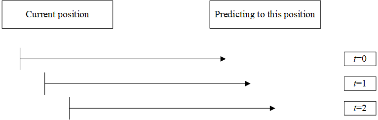
Receding horizen
It means that we continually update our predictions and decision making to take account of the most recent target and measurement data.
One effect is that the prediction horizon is always relative to the current position and recedes away from the viewer as the viewer moves forward.
Feedback from MPC
In MPC, the continual update prediction and decision making based on the measurement data introduces the feedback. (Measurement introduces feedback.)
- Measurement is a core part of a feedback loop
- decision based on measurement are the second core part
Predictive control incorporates both.
Modelling
Modelling is a core part of prediction control. People can predict based on experience, same idea, in order to make prediction, the behaviors of a system should be clear and the model is required.
However, here comes the problem, what is an appropriate prediction model?
Modelling requirements
- Easy to form prediction - ideally linear
- Easy to identify model parameters
Accurate prediction: steady-state, fast transients, mid-response……
The simplest model gives accurate prediction is usually the best.
But it’s OK if the model is not that accurate, because we have feedback to deal with the small error.
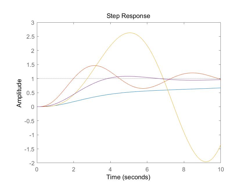
Performance index
We could give out descriptions about what constitutes good or bad, for example, we use SLOW, OSCILLATORY, UNSTABLE, IDEAL to describe the step response.
When we talk about performance index, we need to ask the following questions:
1. What is the performance index for?
In order to decide which input trajectory, we need a precise numeric definition of ‘best’, so the performance index is a numerical definition of what is the best. However, it should be note that the performance index is still have some contradiction with real situation.
2. How should the performance index be designed?
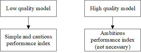
The index should be simple, you should only increase the complexity where the benefits is clear. For example:
With the increase of the experience, people can do more complex activities and give out more challenging performance indices, because our internal model is better through experience.
Typically quadratic performance is used, because:
- It give us well conditioned optimization
- Unique minimum
- smooth behaviours (unlike 1-norm or inf-norm)
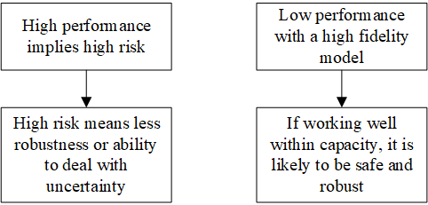
3. How should we make trade offs between optimal and safe/robust performance?
Degree of freedom (DOF)
DOF describes the complexity of the input predictions, it is closely linked to the performance index. There is no point to use high DOF with a highly performance demanding if the model is poor, it’s just like asking a beginner to play like a master!
| The useful num of DOF is related to the prediction accuracy |
An ill-posed performance index is shown below:
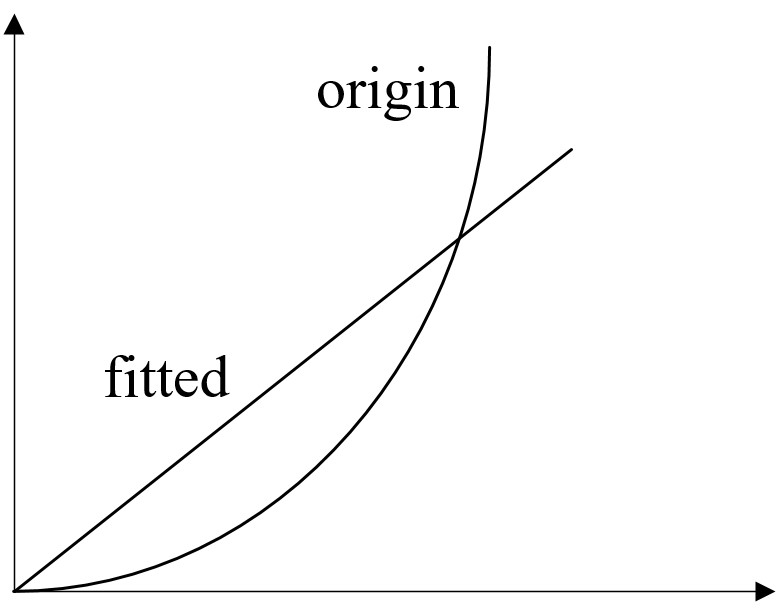
Try to fit a second order curve with one DOF, BAD!! One degree of freedom can only be applied to simple target
In MPC, an ill-posed performance index means that a low prediction horizon (can not predict further events) compared to the system dynamic and use numerous DOF to optimal tracking with that horizon. With low prediction horizon, one cannot fully anticipate the consequence of ones actions, so the planned actions maybe poor.
Constraint handling
One major advantage of predictive control is that it embeds constraints to strategy. It’s critical to getting effective and robust close-loop behavior. We should know that:
- The proposed input trajectory is optimal only if it satisfies constraints
- More typical control strategy treat constraints after thought (like PID)
Example: overshooting
In some situation, overshooting is a disaster (like the chemical tank level control, if overshooted, the chemical spills everywhere! ), it means we lost control of the system and make explosion.
In MPC, the constraints (flow, power or speed limitations) are embedded, which means that it will not propose input flows that allow overshooting, the response time may become slower, but much more safer. In PC, the input is limited to 100% and will not allow earlier input choices which make the system unstable
Multivariable (MIMO)
In MIMO system, often changing one input changes all the outputs, therefore we need an control law consider all the I/Os. One advantage of MPC is that we consider about the interaction, although we need to express the algorithm in mathematical form.
How MPC works
Mathematical form about MPC
Basic of MPC
The first thing we need to know that the implementation of MPC is usually in discrete time1. Meanwhile, due to the limitations of physical world, there are constrains:
so in practical control system, we need to solve a constrained LQR problem, now let’s convert infinite-time limit to a $N$ step finite-time limit. Then our optimal problem becomes a set of linear equations with variables ${\mathrm{x}(1), \mathrm{x}(2), \ldots, \mathrm{x}(\mathrm{N}) ; \mathrm{u}(0), \mathrm{u}(1), \ldots, \mathrm{u}(\mathrm{N}-1)}$, the initial state is $x(0)=x_0$. Now we give out the goal of MPC
Goal: find the best control sequence over a future horizon of $N$ steps
Linear MPC (equals to linear state-feedback!)
Unconstrained case
Let’s consider our linear prediction model:
The relation between input and states is:
and the performance index is (cost function, see ):
Goal: find a sequence $z^*$ to minimize cost function $J$. See LQG regulator.
Now let’s take a look at the cost function
the optimum is obtained by zeroing the gradient
and hence the solution is:
Unconstrained linear MPC = linear state-feedback!
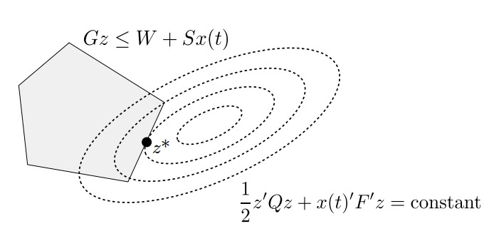
constrained case
Still the prediction model above, this time we add input and output constraints to enforce, our control problem becomes
write as condensed form:
- Input constraints $u{\min } \leq u{k} \leq u_{\max }$
- Output constraints $
y{k}=C A^{k} x{0}+\sum{i=0}^{k-1} C A^{i} B u{k-1-i} \leq y_{\max }, k=1, \ldots, N
$
Linear MPC algorithm
At each sampling time $t$:
- measure (or estimate) the current state $x(t)$
- Get the solution $z^=\left[\begin{array}{c}{u_{0}^} \ {u{1}^*} \ {\vdots} \ {u{N-1}^*}\end{array}\right]$ of the QP
- Apply only $u(t)=u^_0$, discarding the remaining optimal inputs $u^1,…,u^*{N-1}$
Application
Explicit MPC Control of a Single-Input-Single-Output Plant3
This subsection is mainly a summarization about reference 3.
Plant design
The linear open-loop dynamic model is a double integrator.
1 | plant = tf(1,[1 0 0]); |
MPC design
1 | Ts = 0.1; |
Psets the prediction horizon steps, specified as a positive integer. The product ofPredictionHorizonandTsis the prediction time; that is, how far the controller looks into the future.Control horizon, specified as one of the following:
- Positive integer, m, between
1and p, inclusive, where p is equal toPredictionHorizon. In this case, the controller computes m free control moves occurring at times k through k+m-1, and holds the controller output constant for the remaining prediction horizon steps from k+m through k+p-1. Here, k is the current control interval. - Vector of positive integers [m1, m2, …], specifying the lengths of blocking intervals. By default the controller computes M blocks of free moves, where M is the number of blocking intervals. The first free move applies to times k through k+m1-1, the second free move applies from time k+m1 through k+m1+m2-1, and so on. Using block moves can improve the robustness of your controller. The sum of the values in
ControlHorizonmust match the prediction horizon p. If you specify a vector whose sum is:- Less than the prediction horizon, then the controller adds a blocking interval. The length of this interval is such that the sum of the interval lengths is p. For example, if p=
10and you specify a control horizon ofControlHorizon=[1 2 3], then the controller uses four intervals with lengths[1 2 3 4]. - Greater than the prediction horizon, then the intervals are truncated until the sum of the interval lengths is equal to p. For example, if p=
10and you specify a control horizon ofControlHorizon=[1 2 3 6 7], then the controller uses four intervals with lengths[1 2 3 4].
- Less than the prediction horizon, then the controller adds a blocking interval. The length of this interval is such that the sum of the interval lengths is p. For example, if p=
- Positive integer, m, between
Specify actuator saturation limits as MV constraints.
1 | mpcobj.MV = struct('Min',-1,'Max',1); |