Linear Quadratic Gaussian Regulator

Life is short, always choose the best

In this article, we are going to give a summarization about the LQG regulator. Like the pole placement control law, the LQG can also guide us to determine the parameters in a full state-feedback controller.

Prerequisite knowledge

Linear quadratic regulator

Before talking about the LQG regulator, let’s first discuss about LQR since it is a simplified form about LQG. (without Gaussian noises)

A simple problem

Consider you are going to a park (desired state) from your home (initial state), you have several choices:

	Time	Cost
Car	20min	7
Bike	75min	0
Bus	30min	2
Airplane	4min	400

If you want speed, choose airplane, if you have little money, choose bike, or you can make a compromise between time and money to take a car or a bus.

Define a cost function:

$\begin{equation} J=Qt+Rm \end{equation} \label{JQtRm}$

where $t$ is time and $m$ is money, $Q$ and $R$ are two weight matrix. Based on the cost function, we make the optimal choose. Remember that the cost is strongly related to the weight matrix.

LQR in control system

Now let’s consider our control system, we want to make a balance between the performance and actuator effort (energy). So we set up a cost function of the performance ($x$) and the effort ($u$):

$\begin{equation} J=\int_{0}^{\infty}\left(x^{\top} Q x+u^{\top} R u\right) d t \end{equation}$

by solving the LQR problem, it returns the gain matrix $K$ that produce the lowest cost given the dynamic system. We penalizing the performance by $Q$ and penalizing the effort by $R$. Thus the function of LQR is:

Given a system function with initial state, by providing a proper control quantity, the system can be transfered to a desired terminal state with lowest cost.

Intuitive understand of the cost in system

Performance is judged by the state $x$. Suppose that our system is at a none zero initial state, we want it to get to the zero state. The faster it return to zero, the better the performance is and the lower the cost. How to measure how quickly to return the desired state is to looking at the area under the curve, this is what the integral doing, a curve with less area means a better performance. Since the state can be either positive and negative, we square the value to keep positive.

图片名称

The operation above turns our cost function to a quadratic function with a form of $z=x^2+y^2$, it has a definite minimum value (Great!). Now let’s consider the form of $Q$, the $Q$ needs to be positive definite thus $x^{\top} Q x>0$, normally it is a diagonal matrix:

$\begin{equation} \left[\begin{array}{ll}{x_{1}} & {x_{2} \dots x_{n}}\end{array}\right] \begin{bmatrix} q_1 & & & 0\\ & q_2 & & \\ & & \ddots & \\ 0& & & q_3 \end{bmatrix} \left[\begin{array}{c}{x_{1}} \\ {x_{2}} \\ {\vdots} \\ {x_{n}}\end{array}\right] \end{equation}$

Similarly, the $R$ matrix can penalize the input $u$, we can rewrite the equation as follows:

$\begin{equation} \left[\begin{array}{ll}{x^{\top}} & {u^{\top}}\end{array}\right]\left[\begin{array}{ll}{Q} & {0} \\ {0} & {R}\end{array}\right]\left[\begin{array}{l}{x} \\ {u}\end{array}\right] \end{equation}$

Now we can make a judgment, for example, if an actuator $u_i$ is really expensive, we can penalizing it by increasing $r_i$, if lower error $x_i$ is important, you can increasing the $q_i$.

Mathematical form and solution about LQR

For a continuous-time linear system, defined on $t \in\left[t{0}, t{1}\right]$, described by:

$\begin{equation} \dot{x}=A x+B u \end{equation}$

with a quadratic cost function defined as:

$\begin{equation} J=x^{\top}\left(t_{1}\right) F\left(t_{1}\right) x\left(t_{1}\right)+ \int_{t_{0}}^{t_{1}}\left(x^{\top} Q x+u^{\top} R u+2 x^{\top} N u\right) d t \end{equation}$

in which:

$x^{\top}\left(t{1}\right) F\left(t{1}\right) x\left(t_{1}\right)$ is an index about steady state
$\int{t{0}}^{t_{1}}x^{\top} Q x d t$ is an index about transient process
$\int{t{0}}^{t_{1}}u^{\top} R u d t$ is an index about system energy

The feedback control law that minimizes the value of the cost is:

$\begin{equation} u=-K x \end{equation}$

Solution: Now let’s solve the LQR problem, taking discrete LQR as an example, we use Lagrangian multiplier method to solve it, given the optimization problem:

$\begin{equation} \begin{aligned} &J=X^{\top}(N)Q_0X(N)+\sum_{i=0}^{N-1}[X^{\top}(i)QX(i)+U^{\top}(i)RU(i)]\\ s.t.\quad &X(0)=X_0\\ &X(k+1)=AX(k)+BU(k) \end{aligned} \end{equation}$

Step1: Create Lagrangian function to combine the cost function and constrains.

Using the Lagrangian multiplier $\lambda$, we can create a function combine the cost function and constrains.

$\begin{equation} \begin{aligned} J_l&=X^{\top}(N)Q_0X(N)+\sum_{i=0}^{N-1}[X^{\top}(i)QX(i)+U^{\top}(i)RU(i)]+2\sum_{i=0}^{N-1}\lambda^{\top}(i+1)[AX(i)+BU(i)-X(i+1)]\\ &=X^{\top}(N)Q_0X(N)-2\lambda^{\top}(N)X(N)+\sum_{i=1}^{N-1}[H(i)-2\lambda^{\top}(i)X(i)]+H(0) \end{aligned} \end{equation}$

where

$\begin{equation} \begin{aligned} H(k)=X^{\top}QX+U^{\top}RU+2\lambda^{\top}(i)X(i)[AX+BU] \end{aligned} \end{equation} \label{XtopQX}$

Step2: Find the extreme point we of the cost function

finding the minimum of $J_l$ is to find the extreme point of $J_l$, thus we need to satisfy the following conditions:

$\begin{equation} \left\{ \begin{aligned} \frac{\partial J_{l}}{\partial X(k)}&=2 Q X(k)+2 A^{T} \lambda(k+1)-2 \lambda(k)=0 \\ \frac{\partial J_{l}}{\partial U(k)}&=2 R U(k)+2 B^{T} \lambda(k+1)=0 \\ \frac{\partial J_{l}}{\partial \lambda(k+1)}&=2 A X(k)+2 B U(k)-2 X(k+1)=0 \end{aligned} \right. \end{equation}$

meanwhile, the final state satisfies:

$\begin{equation} \frac{\partial J_{l}}{\partial X(N)}=2 Q_{0} X(N)-2 \lambda(N)=0 \end{equation}$

Step3: Solving the control law and feedback gain

With a series transformation and solving a Riccati function, we get the control law

$\begin{equation} U(k)=-R^{-1} B^{T} A^{-T}[S(k)-Q] X(k) \end{equation}$

and feedback gain

$\begin{equation} K=R^{-1} B^{T} A^{-T}[S(k)-Q] \end{equation}$

That is the feedback regulator we need.

In Matlab, give $Q$ and $R$, run

1	K = lqr(A,B,Q,R)

you get the optimal gain set. With LQR, we don’t place poles, instead, we choose $Q$ and $R$, now here’s the question, what is a proper $Q$ and $R$, it can based on our intuition and knowledge about the system, Or we can start with $Q$ and $R$ equals to identity matrix. Here we summarize the influence of $Q$ and $R$ to the system.

	Overshoot	Setting time	Energy consumption
Increasing $Q$	decreasing	decreasing	increasing
Increasing $R$	increasing	increasing	decreasing

Difference of LQR and pole placement

Basically, the LQR and pole placement controllers have the exactly the same structure, so the implementation of $K$ is the same, but how we choose $K$ is different.

In pole placement, we solve for $K$ by choosing pole locations.
In LQR, we find the optimal $K$ by choosing characteristics.

Linear quadratic estimator

Filtering, Prediction, and Smoothing³

There are three general types of estimators for the LQG problem:

Predictors: use prior observations strictly $t{obs}<t{est}$
Filter: use observations up to and including the time that the state of the dynamic system is to be estimated $t{obs}\leq t{est}$
Smoother: use observations beyond the estimation time $t{obs}>t{est}$

Kalman Filter

The Kalman filter is an optimal algorithm for state estimation, it will help us to reconstruct the state of a dynamic system uses a series measurements observed over time, containing statistical noise and other inaccuracies, and produces estimates of unknown variables that tend to be more accurate than those based on a single measurement alone. For more information about Kalman filter, please refer to Kalman filter for this section.

Linear quadratic Gaussian regulator

Mathematical description of the problem

Let’s concern a linear system driven by addictive white Gaussian noise ($N(0,\Sigma)$), consider a continuous-time linear dynamic system with disturbance and measurement noise:

图片名称

$\begin{equation} \begin{aligned} \dot{\mathbf{x}}(t) &=A(t) \mathbf{x}(t)+B(t) \mathbf{u}(t)+\mathbf{v}(t) \\ \mathbf{y}(t) &=C(t) \mathbf{x}(t)+\mathbf{w}(t) \end{aligned} \end{equation}$

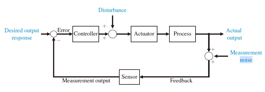
here the $\mathbf{v}(t)$ and $\mathbf{w}(t)$ are the system noise and measurement noise. The objective of LQG is to find the control input history $\mathbf{u}(t)$ which at any time only depends linearly on the past measurement $\mathbf{y}\left(t^{\prime}\right), 0 \leq t^{\prime}<t$ such that the following cost function is minimized:

$\begin{equation} \begin{array}{l}{J=\mathbb{E}\left[\mathbf{x}^{\mathrm{T}}(T) F \mathbf{x}(T)+\int_{0}^{T} \mathbf{x}^{\mathrm{T}}(t) Q(t) \mathbf{x}(t)+\mathbf{u}^{\mathrm{T}}(t) R(t) \mathbf{u}(t) d t\right]} \\ {F \geq 0, \quad Q(t) \geq 0, \quad R(t)>0}\end{array} \end{equation}$

where $\mathbb{E}$ denotes the expected value $T$ may be either finite or infinite, if infinite, the first term $\mathbf{x}^{\mathrm{T}}(T) F \mathbf{x}(T)$ can be ignored.

Here we gives out a simple explanation about why we regard the noise as Gaussian. A Gaussian noise means that if we added multiple noises, it will still obey the Gaussian distribution.

Regulator design

Now let’s design the LQG regulator, the LQG controller that solves the LQG control problem is specified by the following equations:

$\begin{equation} \begin{array}{l}{\dot{\hat{\mathbf{x}}}(t)=A(t) \hat{\mathbf{x}}(t)+B(t) \mathbf{u}(t)+L(t)(\mathbf{y}(t)-C(t) \hat{\mathbf{x}}(t)), \quad \hat{\mathbf{x}}(0)=\mathbb{E}[\mathbf{x}(0)]} \\ {\mathbf{u}(t)=-K(t) \hat{\mathbf{x}}(t)}\end{array} \end{equation}$

where matrix $L(t)$ is the gain of the state estimator (Kalman gain) while $K(t)$ is the feedback gain.

Solve for $L(t)$

$L(t)$ is computed from $A(t),C(t),V(t),W(t)$ and finally $\mathbb{E}\left[\mathbf{x}(0) \mathbf{x}^{\mathrm{T}}(0)\right]$ through the following associated matrix Riccati differential equation:

$\begin{equation} \begin{array}{l}{\dot{P}(t)=A(t) P(t)+P(t) A^{\mathrm{T}}(t)-P(t) C^{\mathrm{T}}(t) W^{-1}(t) C(t) P(t)+V(t)} \\ {P(0)=\mathbb{E}\left[\mathbf{x}(0) \mathbf{x}^{\mathrm{T}}(0)\right]}\end{array} \end{equation}$

Given the solution $P(t), 0 \leq t \leq T$ the Kalman gain equals

$\begin{equation} L(t)=P(t) C^{\mathrm{T}}(t) W^{-1}(t) \end{equation}$

Solve for $K(t)$

Similar to solving for $L(t)$, the feedback gain $K(t)$ can be determined by the following Riccati differential equation:

$\begin{equation} \begin{array}{l}{-\dot{S}(t)=A^{\mathrm{T}}(t) S(t)+S(t) A(t)-S(t) B(t) R^{-1}(t) B^{\mathrm{T}}(t) S(t)+Q(t)} \\ {S(T)=F}\end{array} \end{equation}$

Given the solution $S(t), 0 \leq t \leq T$ the feedback gain equals

$\begin{equation} K(t)=R^{-1}(t) B^{\mathrm{T}}(t) S(t) \end{equation}$

The Riccati differential equation of $L(t)$ solves the linear–quadratic estimation problem (LQE) while the second LQR problem, together they solve the linear-quadratic Gaussian control problem. So the LQG problem separates into the LQE and LQR problem that can be solved independently. Therefore, the LQG problem is called separable.

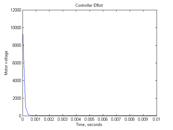
Application: LQG regulator design for a inverted pendulum system

In this section we will design a LQG regulator for a noise added inverted pendulum system which is basically an extended part of .