State-space, feedback and estimators

Abstract

Some reading notes about state-space, and feedback and estimators in state space method basically from chapter 8 of $\textit{Linear system theory and design}$ ¹.

State-space

What is a state-space model?

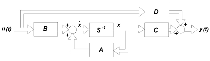
A state-space model, according to reference 2², is a model uses state variables to describe a system by a set of first-order differential or difference equations, rather than by one or more nth-order differential or difference equations. In state-space models, we reconstruct state variables from input-output data rather than measure them directly.

Here’s the mathematical form and block diagram of SS model.

$$\begin{aligned} \label{equ1} \dot x(t)&=Ax(t)+Bu(t)+ \tilde K w(t)\\ y(t)&=Cx(t)+Du(t)+w(t)\\ x(0)&=x0 \end{aligned}$$

Why we need state-space model

• Can be used for Linear and nonlinear systems.
• For both SISO and MIMO systems.
• First order ODE’s means perfect for analysis
• working in time domain

State-space and transfer functions: conversion

SS to TF

$$\begin{aligned} \dot x(t)&=Ax(t)+Bu(t)\\ y(t)&=Cx(t)+Du(t)\\ x(0)&=\textbf 0 \end{aligned}$$

• Laplace transfer

$$\begin{aligned} sX(s)&=AX(s)+BU(s)\\ Y(s)&=CX(s)+DU(s)\\ \end{aligned}$$

• Shift Item

$$H(s)=\frac{Y(s)}{U(s)}=C\Phi(s)B+D=C(sI-A)^{-1}B+D$$

In Matlab (God I really like Matlab)

[n,d]=ss2tf(A,B,C,D)

TF to SS

$$H(s)=\frac{Y(s)}{U(s)}=\frac{b_0}{s^n+a_1s^{n-1}+\cdots +a_{n-1}s+a_n}$$

• Shift Item and create differential equation

$$y^{(n)}+a_1y^{(n-1)}+\cdots+a_{n-1}\dot y+a_ny=u$$

• Choose state variables

$$\begin{bmatrix} x_1=y\\ x_2=\dot y\\ \vdots \\ x_n=y^{(n-1)} \end{bmatrix}\rightarrow \begin{bmatrix} \dot x_1=\dot y\\ \dot x_2=\ddot y\\ \vdots \\ \dot x_n =y^{(n)} \end{bmatrix}$$

• Write as ss form

State Feedback

What is state feedback

Consider a simple open loop SISO ss euqation:

$$\begin{aligned} \dot x(t)&=\textbf Ax(t)+\textbf bu(t)\\ y(t)&=\textbf Cx(t)\\ \end{aligned}$$

We want use $u(t)$ to change system dynamics, so we introduce linear state feedback with gain $\textbf k$:

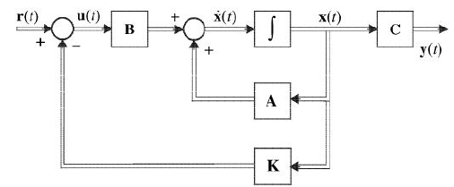
Now the input u is given by $u(t)=r(t)-\textbf kx(t)$ and our ss equation becomes:

$$\begin{aligned} \dot x(t)&=(\textbf A-\textbf {bk})x(t)+\textbf bu(t)\\ y(t)&=\textbf Cx(t)\\ \end{aligned}$$

Why we need state feedback

From the equations above we replace $\textbf A$ with $\textbf{A-bk}$, we know that $\textbf A$’s eigenvalues give the open-loop system poles, by selecting proper $\textbf K$, we can place the eigenvalues in any positions we what.

• $\mathscr{Theorem}\ 1$

If n-dimensional ss equation is controllable, the eigenvalues of $\textbf{A-bk}$ can be arbitrarily assigned.

How do we design a proper state feedback

Method 1: According to desired pole placement

To apply pole placement method, first we need to clear how the pole influence the system, please refer to another article:

In Matlab, we give system parameters and desired eigenvalues, the place function will give out the feedback gains. (We choose desired eigenvalues through system performance)

a=[0 1 0 0; 0 0 -1 0; 0 0 0 1;0 0 5 0]
b=[0;1;0;-2]
p=[-1.5+0.5j -1.5-0.5j -1+j -1-j]
k = place(a,b,p)   % Or use the acker function

Method 2: Solving Lyapunov Equation

Same question as above, we want a proper $\textbf k$.

• First, we need a matrix $\textbf F$ according to eigenvalues
• Next we select an $1\times n$ vector $\bar {\textbf{k}}$ makes $(\textbf F,\bar {\textbf{k}})$ observable
• Then we solve the unique $T$ in Lyapunov equation $\textbf{AT-TF=b}\bar {\textbf{k}}$
• Finally we compute feedback gain $\textbf k=\bar {\textbf{k}}\textbf T^{-1}$

Matlab codes

a=[0 1 0 0; 0 0 -1 0; 0 0 0 1;0 0 5 0];
b=[0;1;0;-2];
f = [-1 1 0 0; -1 -1 0 0; 0 0 -1.5 0.5; 0 0 -0.5 -1.5];
kb=[1 0 1 0];
k=kb*inv(t)

Method 3: LQR Method

The LQR method is an optimal control method which goal is to find the controller that minimizes a quadratic cost function subject to the linear system dynamics. It’s assumed that

• There is no noise
• The full system is observerable

The mathematical form of LQR is:

$$\begin{aligned} &\min \limits_{u(\cdot )}\int_{0}^{T}(x^TQx+u^TRu)dt + x(T)^TQ_fx(T)\\ s.t.\ \ &\dot x=Ax+bu\\ &y=x\\ &x(0)-Given \end{aligned}$$

The optimal controller for the LQR problem is a linear feedback controller with a form of

$$u(t)=\textbf Kx(t)$$

State Estimator

What is a state estimator

A state estimator or observer is a device generates an estimate of the state. We hope that the output of the estimator is just the same as the behavior of the plant.

Open loop state estimator

Basic structure

First let’s take a look at the open loop state estimator:

If we know $\textbf A $ and $\textbf b$, we can duplicate the system as:

$$\dot {\hat{x}}(t)=\textbf A\hat x(t)+\textbf bu(t)$$

The estimation error is $\tilde{x}(k)=A^{k}(x(0)-\hat{x}(0))$, this is not ideal because:

• The dynamics of the estimation error are fixed by the eigenvalues of A and cannot be modified
• The estimation error vanishes asymptotically if and only if A is asymptotically stable²

Disadvantages:

• initial state must be computed and set each time we use estimator
• There will be a difference between $x(t)$ and $\hat x(t)$

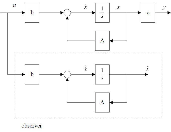
Close loop state estimator (Luenberger observer)

We modify the estimator in which the output $y(t)=c{\textbf x}(t)$ is compared with $c\hat{\textbf x}(t)$, the difference is used as a correlation term. If difference is zero, nothing to do. If the difference is nonzero and gain $\textbf l$ is proper designed, the difference will drive the estimated state to actual state.

$$\dot {\hat{\textbf x}}(t)=\textbf A\hat {\textbf x}(t)+\textbf bu(t)+\textbf l(y(t)-\textbf c\hat{\textbf x}(t))$$

Let’s define $\textbf e(t)$ is the evaluated error of state estimation

$$\begin{equation} \begin{aligned} \textbf e(t):&=\textbf x(t)-{\hat{\textbf x}}(t)\\ \dot{\textbf e}(t)&=\dot{\textbf x}(t)-\dot{\hat{\textbf x}}(t)\\ &=\textbf {Ax}(t)+\textbf bu(t)-\textbf A\hat {\textbf x}(t)-\textbf bu(t)-\textbf l(y(t)-\textbf c\hat{\textbf x}(t))\\ &=(\textbf A-\textbf l\textbf c)(\textbf x(t)-{\hat{\textbf x}}(t))\\ &=(\textbf A-\textbf l\textbf c)\textbf e(t) \end{aligned} \end{equation} \label{etxtxh}$$

This is a first order difference function, by choosing a proper $L$, we can stabilize $(\textbf A-\textbf l\textbf c)$, the solution is an exponential function, thus the state error tends to zero with an exponential form, thus the estimation is unbiased.

From equation $\eqref{etxtxht}$ we can also notice that it doesn’t contain any control quantity, thus it is uncontrollable. However, as long as the system is stable, the estimation error tends to zero if the roots of the characteristic equation $\det(s\textbf I-\textbf A+\textbf l\textbf c)$ fall into the left half plane.

Observer design

x=[-1;1]; % initial state
xhat=[0;0]; % initial estimate

XX=x;
XXhat=xhat;
T=40;
UU=.1*ones(1,T); % input signal

for k=0:T-1,
    u=UU(k+1);
    y=C*x+D*u;
    yhat=C*xhat+D*u;
    
    x=A*x+B*u;
    xhat=A*xhat+B*u+L*(y-yhat);
    
    XX=[XX,x];
    XXhat=[XXhat,xhat];
end

plot(0:T,[XX(1,:);XXhat(1,:)]);

Why we need a state estimator

Ideally, the state variables are all available for feedback. In practice, some variables are not accessible. So we introduce observers to the system, for example, in self-driving, we have GPS, IMU, et al. as observers.

How to design a state estimator

The equation $\dot{ \textbf{e}}(t)=(\textbf A-\textbf l\textbf c)\textbf e(t)
$ governs the estimation error. If all eigenvalues of $(\textbf A-\textbf l\textbf c)$ can be arbitrarily assigned, we can control the rate for $\textbf e(t)$ to approach zero, so the feedback gain of $\textbf l$ help us to reduce the difference between actual state and observed state. Since we want the dynamics of the observer to be much faster than the system itself, we need to place the poles at least five times farther to the left than the dominant poles of the system.

p=[-1.5+0.5j -1.5-0.5j -1+j -1-j]
L = place(A',C',p*10);

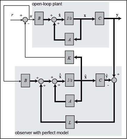
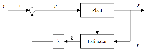
Feedback from estimated states

Now let’s combine the feedback with state estimator, our state variables are not available for feedback, so we design a state estimator to get the observed variables.

It can be proved that the feedback and estimator are independent and can be carried out independently. This is called the separation property.

Application: State feedback control of a inverted pendulum system

This section is mainly based on a short tutorial from reference ³.

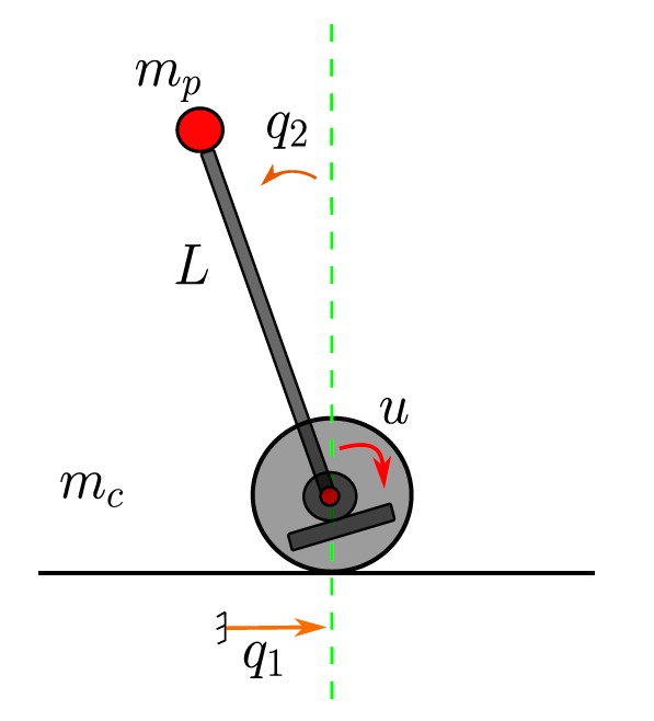
Problem setting

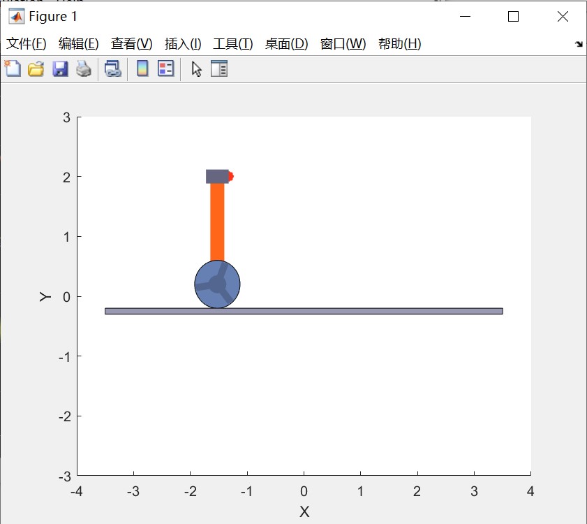
Suppose we have a Pendulum-Cart system to be controlled shown below

The overall objective will be broken down into the following tasks:

• Linear dynamic system modeling
• System analysis
• Controller designing in SS
• State observer designing and investigating in close loop
• Discretization

Linear dynamic system modeling

We shall not focus too much on the modeling process, here we give out the linear model of inverted pendulum directly:

$$\begin{aligned} \textbf{x} &= \begin{pmatrix} q_1\\ q_2\\ \dot q_1\\ \dot q_2 \end{pmatrix} \\ \dot {\textbf{x}} &= \textbf A\textbf{x}+\textbf bu \end{aligned}$$

Let $q_1$ (position) and $q2$ (angular) be the system output, $\textbf A$ and $\textbf b$ is:

$$\begin{aligned} \textbf{A} = \begin{pmatrix} 0& 0& 1 &0\\ 0& 0& 0 &1\\ 0 &\frac{gm_p}{m_c} & \frac{-d_1}{m_c} & \frac{-d_2}{Lm_c}\\ 0 &\frac{g(m_c+m_p)}{Lm_c} & \frac{d_1}{Lm_c} &-\frac{d_2(m_c+m_p)}{L^2m_cm_p} \end{pmatrix} ,\ \ \ \textbf{B} = \begin{pmatrix} 0\\ 0\\ \frac{1}{m_c}\\ \frac{1}{Lm_c} \end{pmatrix} \end{aligned}$$

where: $m_c = 1.5,m_p=0.5,g=9.82,L=1,d_1=d_2=0.01$.

clc;
clear;
close all;

mc = 1.5;
mp = 0.5;
g  = 9.82;
L  = 1;
d1 = 1e-2;
d2 = 1e-2;

A  = [0,                   0,          1,                         0;
      0,                   0,          0,                         1;
      0,           (g*mp)/mc,     -d1/mc,                -d2/(L*mc);
      0,(g*(mc + mp))/(L*mc), -d1/(L*mc),-(d2*mc+d2*mp)/(L^2*mc*mp)];
B  = [0; 0 ; 1/mc; 1/(L*mc)];

C   = [1;0;0;0];          % Set q_1 as output
D = 0;

x0 = [0;5*pi/180;0;0];    % Initial state of the integrator

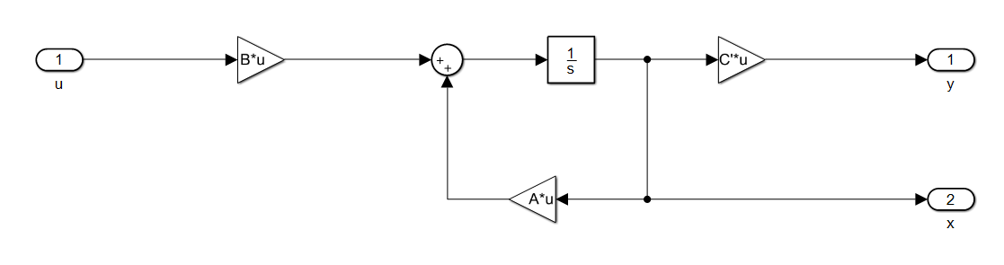
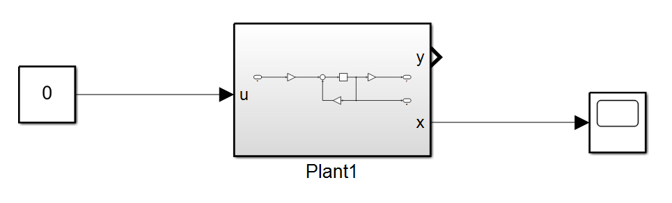
And the plant in simulink is:

System analysis

Given a zero input, the output of the system shows that it’s not stable:

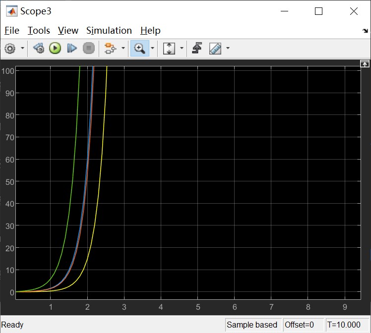
You can also refer to the eigenvalues, the root locus to see the stability of the system.

%% System stability
eig_A = eig(A);      % Eigenvalue of A
pole_A =pole(sys);   % Has a positive pole, not stable

Sc = ctrb(sys);      % Controllability
So = obsv(sys);      % Observability
rank(Sc)             % 4
rank(So)             % 4

Controller designing in SS

First we give out the desire pole we want our system to be set (according to the performance of the system). Based on the desire pole, we can calculate the feedback gain $\textbf K$ (Click here to review state feedback).

%% Controller
des_pole = [-3,-3,-3,-3];
K        = acker(A,B,des_pole);

Or we can apply the LQR method to get the gain (Click here to review LQR methood).:

Q        = eye(4);
R        = 1;
K_lqr    = lqr(A,B,Q,R);

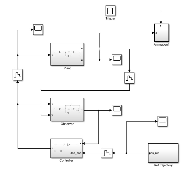
The controller and it’s inner structure is shown below

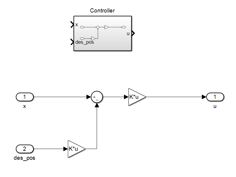
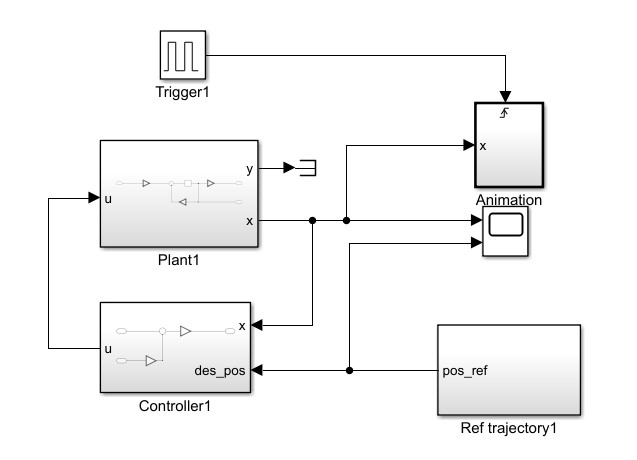
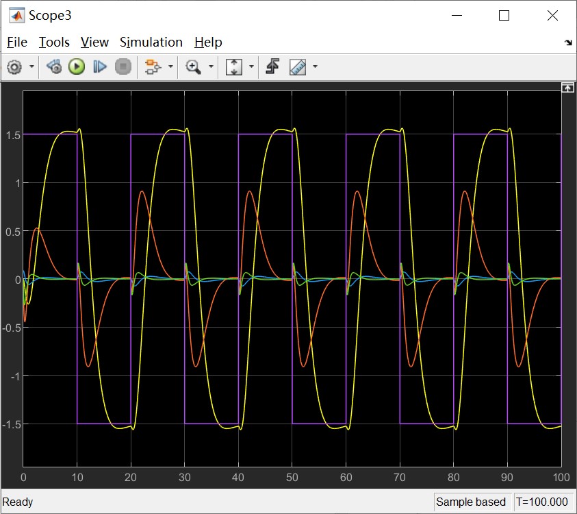
By adding the controller to the system, now we can apply a control behavior to the plant. Given a reference trajectory pulse, we can check the out put of the system. The control system, input and output trajectories and the simulation animation is shown below.

State observer designing and investigating in close loop

So far so good, now let’s further introduce the observer to the system, Click here to review the design process of a state estimator.

L       = acker(A',C,des_pole*10);

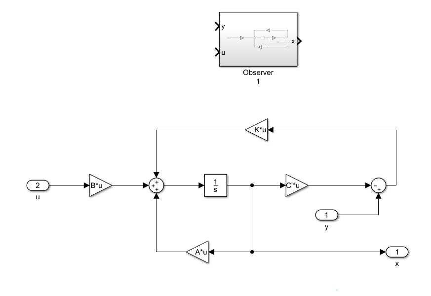
The observer and it’s inner structure is shown below

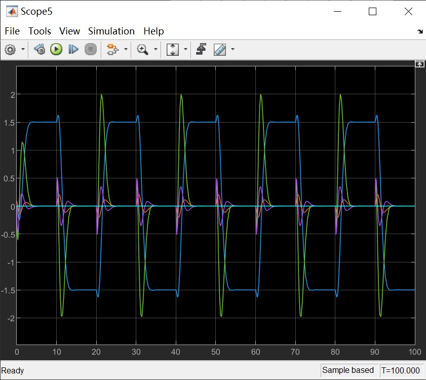
And the output of the observer is quite like the original plant.

Discretization

The final step is to discrete the controller and observer. First we discrete the controller, then the observer.

% discrete 
Ts = 0.1;
sys_d = c2d(sys,Ts);

Ad   = sys_d.a;
Bd   = sys_d.b;
Cd   = sys_d.c;
Dd   = sys_d.d;

des_pole_d = [0.3; 0.3;0.3;0.3];  
K_d = acker(Ad,Bd,des_pole_d);

des_pole_d = [0.3;0.3;0.3;0.3]*0.1;
L_d  = acker(Ad',Cd',des_pole_d);

Then replace the parameters in the system with discrete ones and add zero order holder, change integrator to unit delay model, we get our discrete control system.

reference

---

1. 1.Chen C T. Linear system theory and design[M]. Oxford University Press, Inc., 1998. ↩
2. 2.State estimation and linear observers ↩
3. 3.Matlab documents about ss ↩
4. 4.State Space Control for the Pendulum-Cart System ↩